xpExplosiaFX

xpExplosiaFX is used for the simulation of smoke and fire.

To use xpExplosiaFX, you need a source object (something to burn), which must be located inside the solver boundary.

In addition, there must be an xpExplosiaFX Source tag on the source object.

Solver tab

Untitled

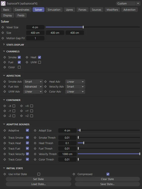
xpExplosiaFX Solver tab.

Voxel Size

This is the voxel size within the boundaries of the solver.

The solver volume is divided into cubes of this size.

Smaller values result in more accurate simulations but are slower to playback and render.

As the voxels get smaller, more particles are required to generate the smoke, etc.

Animation demonstrating Voxel Size settings of 3cm (on the left) and 1cm (on the right), within the solver.

Size

The size of the outer boundary of the solver, shown as a pink box in the viewport.

The simulation always remains within the confines of this box.

Motion Gap Fill

This setting causes extra steps to be added to fill in motion between frames.

If the source object is geometry, the value indicates the density of the infill, not an actual number.

The higher the value, the better the result, but higher values will slow the simulation.

If the source is an X-Particles emitter, the only relevant setting is either 0 or 1.

There is no difference with higher numbers when using particles.

Stats Display

These are some statistics regarding memory use and processing time; they are updated as the simulation runs.

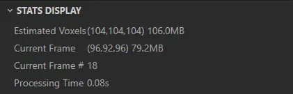
Estimated Voxels

The total number of voxels used and the overall memory requirement.

This will change if the voxel size and/or the solver size changes.

Current Frame

The actual number of voxels used for this frame and the memory requirement.

Current Frame

The current frame being simulated.

Processing Time

The time in seconds to process this frame.

Channels

These checkboxes indicate which channels are used in the simulation.

The default is for smoke, heat and fuel to be checked.

Smoke, Heat, Fuel

In fire simulations, a fire requires fuel to burn and heat to ignite the fuel.

This may then generate smoke, or it may not, and you can turn smoke off if desired.

But if you turn off fuel, there is nothing to burn and you won’t see the fuel or smoke even though there is still heat.

Turn off heat and there’s nothing to ignite the fuel, so you will see nothing happening at all.

As an example, if you have the Display tab set to display fuel and smoke, then you uncheck Smoke in this tab, you will only see the fuel display, as no smoke will be generated.

If you look carefully though, and you have adaptive bounds enabled, you can see that something is happening because the adaptive bounds are visible.

You can see why this is if you change the display to temperature: this shows that you still have heat but no smoke or burning.

Color

If you check this box, to add the color channel to the solver, you can specify a specific color to be used in the display.

To do this, you would also need to turn the Display setting in the Display tab to Color.

UVW

If this box is checked, UVW data is generated so that textures such as noise can be mapped to the simulation for extra detail.

Advection

Advection is the process of the transport of some quantity - e.g. smoke or velocity - through a fluid or gas, by motion.

Smoke Adv, Heat Adv, Fuel Adv, Velocity Adv, UVW Adv, Color Adv

xpExplosiaFX carries out advection for six different properties.

For each one there is a drop-down menu giving a choice of algorithm.

In each case the options are: Smart, Linear and Advanced.

Smart

The slowest algorithm and the most memory-intensive, this is the most detailed of the three and is therefore recommended for smoke advection, for which fine detail is important.

Linear

The fastest algorithm and the best choice for heat advection.

It is also recommended for color and UVW.

Advanced

A slower algorithm, recommended for fuel advection.

Container

The simulation can only take place within the bounds of the solver.

-X, +X, -Y, +Y, -Z, +Z

Checking these individual settings will add a ‘wall’ in the solver, to close that boundary.

Adaptive Bounds

When solving the simulation, you could simply solve each voxel inside the bounds, but that would be slow and inefficient.

Instead, you can solve only those voxels where something is happening, adjusting the volume to be solved as the simulation progressed.

This is what adaptive bounds does.

In general you should leave this enabled unless you require the whole solver volume to be solved each iteration, but doing that will be significantly slower than using adaptive bounds.

Adaptive

Check this box to enable adaptive bounds.

Adapt Size

This is the size of the additional ‘padding’ around each active voxel as the simulation progresses.

In most cases the default setting is fine and there is no need to change it.

Track Smoke, Track Heat, Track Fuel, Track Velocity, Track Color

To adjust the bounds the solver must keep track of some parameter, such as smoke or fuel.

With these settings you can choose which parameters the solver will track.

Smoke Thresh, Heat Thresh, Fuel Thresh, Velocity Thresh, Color Thresh

These are the minimum values of a tracked parameter, which must be present in a voxel before a change in bounds takes place.

If these values are never exceeded, the bounds will never change.

For example, if you track only the heat, the heat value in any voxel must reach the heat threshold level to trigger the adaptive bounds.

If the xpExplosiaFX Source tag has a Heat value set to 100% and you set the threshold in the solver to 1.1 (i.e. 110%), nothing will happen because the threshold will never be exceeded.

But, if you set the tag’s Heat value to 120%, the simulation will run again.

Initial State

With these controls you can run the simulation to a point you like then set the initial state and rewind the animation.

When you play it again, it will start from the point you saved it, rather than from the original start point.

Use Initial State

Check this box to use an initial state once you have set one.

If at any point you want to run the simulation from the beginning but not lose the saved state, uncheck this box.

Compressed

If this setting is enabled, the saved stated will be compressed to save memory.

Set State

Run the simulation to the desired point then stop it and click this button to set the initial state.

This will also automatically check the Use Initial State box for you.

Clear State

Click this button to clear the initial state.

Load State, Save State

If you save a scene file with a set initial state, the state is saved with the file.

You can also save and load the initial state independently, so that you could load the state into a solver in a different scene.

Click the Save State button to save the state to a filename of your choice.

Click the Load State button to load a saved state.

Simulation tab

Untitled

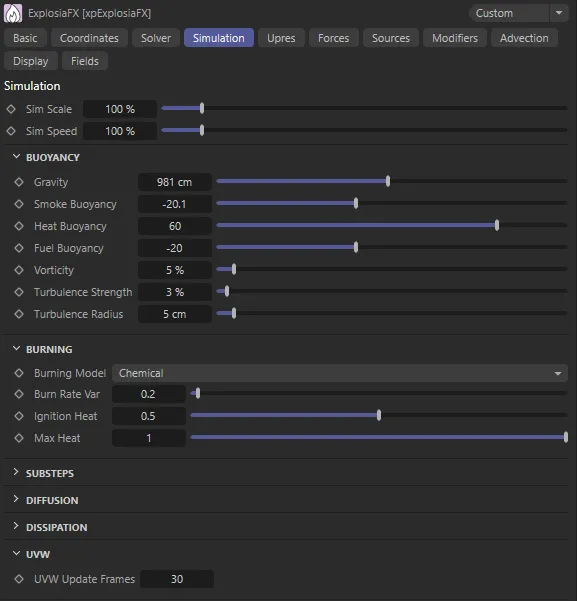
xpExplosiaFX Simulation tab.

Sim Scale

Changing this value alters the resolution of the simulation so that reducing this value results in a larger and faster simulation (within the confines of the solver) but with lower resolution.

A higher value causes a smaller simulation but a more detailed one.

Sim Speed

This is the speed with which the simulation progresses, so the higher this value, the faster it runs.

If you set it too high though, you may see a jerky animation as the appearance seems to jump from one frame to the next.

Buoyancy

Gravity

Gravity is inherent in xpExplosiaFX so an xpGravity modifier is not needed.

This is the gravity strength on the positive Y axis.

You can set negative values to make the smoke flow downwards (negative Y axis).

In this animation, the Gravity is set at 1962cm, on the left, and 300cm, on the right, giving a direct comparison.

Smoke Buoyancy

Smoke rises due to the heat of burning.

This value can reduce or increase the smoke buoyancy, so it will rise slower or faster.

Heat Buoyancy, Fuel Buoyancy

The same as for the smoke buoyancy, but for heat and fuel respectively.

Vorticity

Increasing this value will increase the amount of curl within the simulation.

Turbulence Strength

You can add turbulence to the simulation with this parameter, which controls the strength of the turbulence.

Turbulence Radius

Increasing this value will increase the size of the turbulent areas in the simulation.

Burning

Burning Model

Set as Chemical, by default, this is a drop-down menu containing the various burning models used by xpExplosiaFX.

The model defines how heat, smoke and pressure is generated and dissipated.

The alternative setting is: Custom.

Chemical

This model simulates actual chemical processes inside the burning fuel.

Custom

With this option you can design your own burning model.

Selecting Custom opens up further parameter options, explained below.

Burn Rate Var

This controls the random variation in the rate of burning of fuel, to model fuels of uneven consistency.

The number represents a multiplier to the burn rate, so a variation of 0.0 will produce a relatively even burn, and a variance of 1.0 will cause the burn rate to fluctuate between zero and double its regular amount.

Ignition Heat

This is the threshold value above which burning occurs; if the heat at a given point is greater than the Ignition Heat value, fuel will be burned.

The maximum amount is 1.0, in line with the maximum heat that can exist within a simulation.

Max Heat

The maximum heat value which can be achieved at a given point.

The range is 0.001-1.0, with 1.0 being in line with the maximum heat that can exist within a simulation.

If Max Heat is lower than Ignition Heat then no fuel will burn.

Custom Burning options

If you select Custom from the Burning Model drop-down menu, the interface changes slightly.

You can then use this to design your own burning model.

Experimentation is the key here.

Burn Rate

This setting controls the amount of fuel that burns at any moment in time.

A burn rate of 1.0 will consume 1.0 worth of fuel over the course of one second.

The spline modifies this value based on the existing fuel amount.

Heat Production

How much heat is generated during burning.

This is a multiplier applied to the quantity of fuel burned, as controlled by the Burn Rate parameter.

The spline modifies this value based on the existing fuel amount.

Smoke from Heat, Smoke from Fuel

How much smoke is generated during burning as a result of both heat and fuel.

Both heat and fuel are needed to generate smoke; if one is absent there will be no smoke.

The splines modify these values based on the current heat and fuel respectively.

Gas Expansion

How much pressure is generated during burning.

High pressure will result in smoke, heat and fuel being dispersed over a larger area more quickly.

The spline modifies this value based on the existing fuel amount.

Substeps

CFL

The Courant-Friedrichs-Lewy (CFL) number is important in controlling the accuracy and stability of the simulation.

In this object the ‘CFL’ value is a percentage of the voxel size.

If a simulation appears unstable (e.g. too lively or you see an exploding simulation), try reducing this value and/or increasing the Min Substeps or Max Substeps values.

Both measures will, however, take longer to solve.

Min Substeps, Max Substeps

The solving will only be accurate if particles don’t move beyond a single voxel.

The motion is broken into small times (substeps).

These settings control the minimum and maximum number of time steps that will be used.

Higher values, meaning more substeps, will slow the simulation but make it more accurate.

For very fast moving simulations, they may need to be higher if you notice incorrect simulations or artifacts.

Accuracy

xpExplosiaFX is an iterative solver, refining the calculations each iteration.

More iterations result in a more accurate simulation but will take longer to complete.

The accuracy setting determines how close to ‘exact’ the solution is; the higher it is the more likely it is to reach the maximum number of iterations.

That maximum number is specified in Max Pressure Iter.

Max Pressure Iter

For the most part you can leave this setting alone.

It is used internally as the number of sub-frames used when calculating pressure changes each frame.

If you have a very rapidly changing simulation, such as an explosion, you may need to increase this value.

Diffusion

Diffusion in xpExplosiaFX can be thought of as the rate of movement of a parameter, such as smoke or heat, throughout the solver.

The higher these values are, the greater the even distribution of the parameter and so the less contrast you will see in the result.

In the left-hand solver, all three diffusion values are set at their default of zero. On the right, the Smoke Diffusion is raised to 35, the Heat Diffusion is at 55 and the Fuel Diffusion is at 70, giving a completely different result.

Smoke Diffusion, Heat Diffusion, Fuel Diffusion

The diffusion values for smoke, heat and fuel respectively.

Viscosity

This setting is labelled Viscosity but it is actually another diffusion setting, this time for velocity.

As you might expect, increasing this value smooths out movement and gives the impression of a thicker, more viscous medium.

Dissipation

These values control the dissipation of a parameter, the effect being to reduce it over time.

In this animation, the dissipation settings are at their default of zero on the left. On the right, the Smoke Dissipation is increased to 0.05, the Heat Dissipation to 0.15 and the Fuel Dissipation to 0.85, giving greater controls over the solve.

Smoke Dissipation, Heat Dissipation, Fuel Dissipation

The dissipation values for smoke, heat and fuel respectively.

Fuel Ambient

This is the minimum fuel value in a given voxel which is subject to dissipation.

Smaller values will not be affected by dissipation.

Velocity Damp

This setting acts to reduce velocity over time.

UVW

UVW Update Frames

This is the duration over which the UVW fields recalculate UVW coordinates.

Upres tab

It is often useful to work with low-quality draft settings at the design stage of a simulation; this ensures good viewport feedback, whilst making adjustments to the sim.

However, at some point, the sim quality will need to be increased.

This is done by lowering the voxel size in the solver settings.

The problem can be that more accurate settings can fundamentally change the physics of the sim and it may look quite different from the draft.

Upresing is a way of taking a low quality sim and increasing its simulation accuracy, whilst maintaining the look and flow of the original.

Untitled

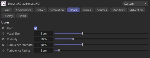
xpExplosiaFX Upres tab.

Upres

Check this box to enable the upres feature.

Voxel Size

The voxel size used for the upres simulation.

Vorticity, Turbulence Strength, Turbulence Radius

These parameters are the same for the upres part of the simulation as found in the Simulation tab.

Forces tab

Although you can apply forces to an xpExplosiaFX solver, using X-Particles modifiers, there is a wind force built in.

Untitled

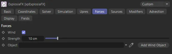
xpExplosiaFX Forces tab.

Wind

Check this box to enable wind.

Strength

The strength of the wind force.

Object

A link field for an xpExplosiaFX Wind object (see below).

You can drag an existing ExplosiaFX Wind object into this field, or click the Add Wind Object button to create a new one.

Add Wind Object

Click this button to create an xpExplosiaFX Wind object.

xpExplosiaFX wind does not require a wind object - simply enabling wind is enough, but it will always blow along the positive Z axis.

If you add a wind object, you can control the wind direction by rotating the xpExplosiaFX Wind object.

ExplosiaFX Wind object

This object looks identical to an xpWind modifier in the viewport.

The object has no parameters than you can alter.

The main use is to rotate it so that it points in the direction you want the wind to blow.

Sources tab

Untitled

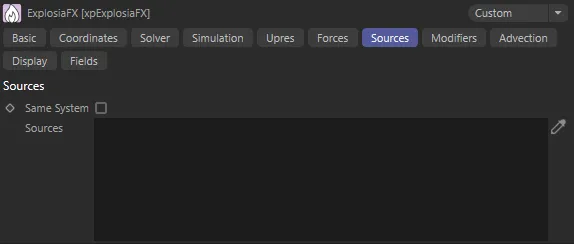
xpExplosiaFX Sources tab.

By default, an object within the bounds of the solver and which has an xpExplosiaFX source tag will be treated as a source for xpExplosiaFX.

If you want to remove a source temporarily without deleting it, you can drag it into this list.

If the object has a yellow check mark icon, it will be used as a source; if it has a blue dash icon, it will not be used.

Same System

If this box is checked, only objects which are child objects of the same System object as the solver will be used as sources.

This setting is ignored if the solver is not in a System object hierarchy.

Sources

The list of source objects.

Modifiers tab

Untitled

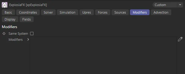
xpExplosiaFX Modifiers tab.

Same System

If this box is checked, xpExplosiaFX will only be affected by modifiers which are child objects of the same System object as the solver.

This setting is ignored if the solver is not in a System object hierarchy.

Modifiers

Drag the required modifiers into this list.

You can temporarily disable a modifier in the list by clicking the yellow check mark icon, to change it to a blue dash.

In this scene, xpFlowField has been dropped into the Modifiers tab and enabled, using the Helix spline, to create a spiraling vector field, to affect the path of the fire.

Advection tab

If you add an emitter to the scene and if you then check the Advect Particles box, the particles from the emitter will be altered in the same way as the parameters such as smoke.

The particle parameters are directly altered by the relevant channel.

For example, if Velocity is set to 100%, the particles take on the velocity in the solver voxels they pass through.

This gives very fluid and natural-looking movement to the particles.

You can turn off the display in the xpExplosiaFX solver, if desired, in which case the solver is, in effect, acting like a particle modifier.

Untitled

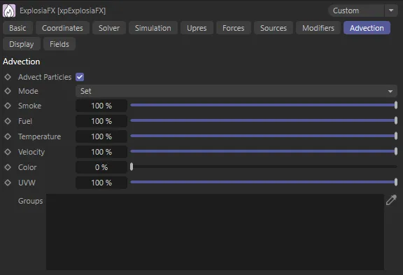
xpExplosiaFX Advection tab.

Advect Particles

Check this box to turn particle advection on.

In this animation, Advect Particles is checked, enabling particle advection with the default settings.

Mode

This is a drop-down menu with two options: Set (the default) and Add.

Set

In this mode, the particle parameter is set each frame with a new value.

Add

In contrast to Set, in this mode, the parameter change is added to the previous value.

This can result in the parameter (such as particle speed) increasing dramatically, which may or may not be desirable.

Smoke, Fuel, Temperature, Velocity, Color and UVW

These settings are the relative effect each of these channels will have on the corresponding particle parameters.

Groups

When a source object is an emitter, you can specify which groups are advected by by dragging the particle group objects into this list.

If the list is empty, all groups emitted by the source emitter are advected.

Display tab

Untitled

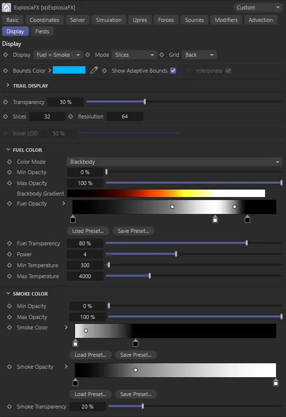
xpExplosiaFX Display tab.

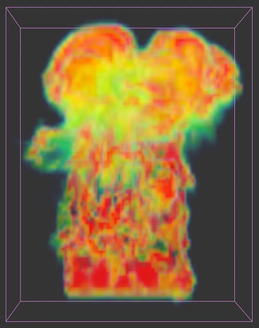
Display

Set as Fuel + Smoke, by default, this drop-down menu controls which channels are shown in the editor.

The other options are: Temperature, Smoke, Fuel, Velocity, Speed and Color.

Each option, apart from Color, has a color gradient and an opacity gradient associated with it for the display.

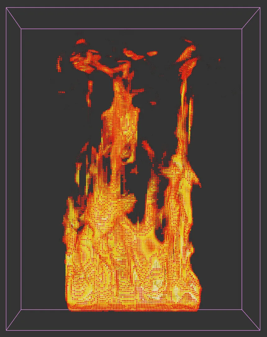
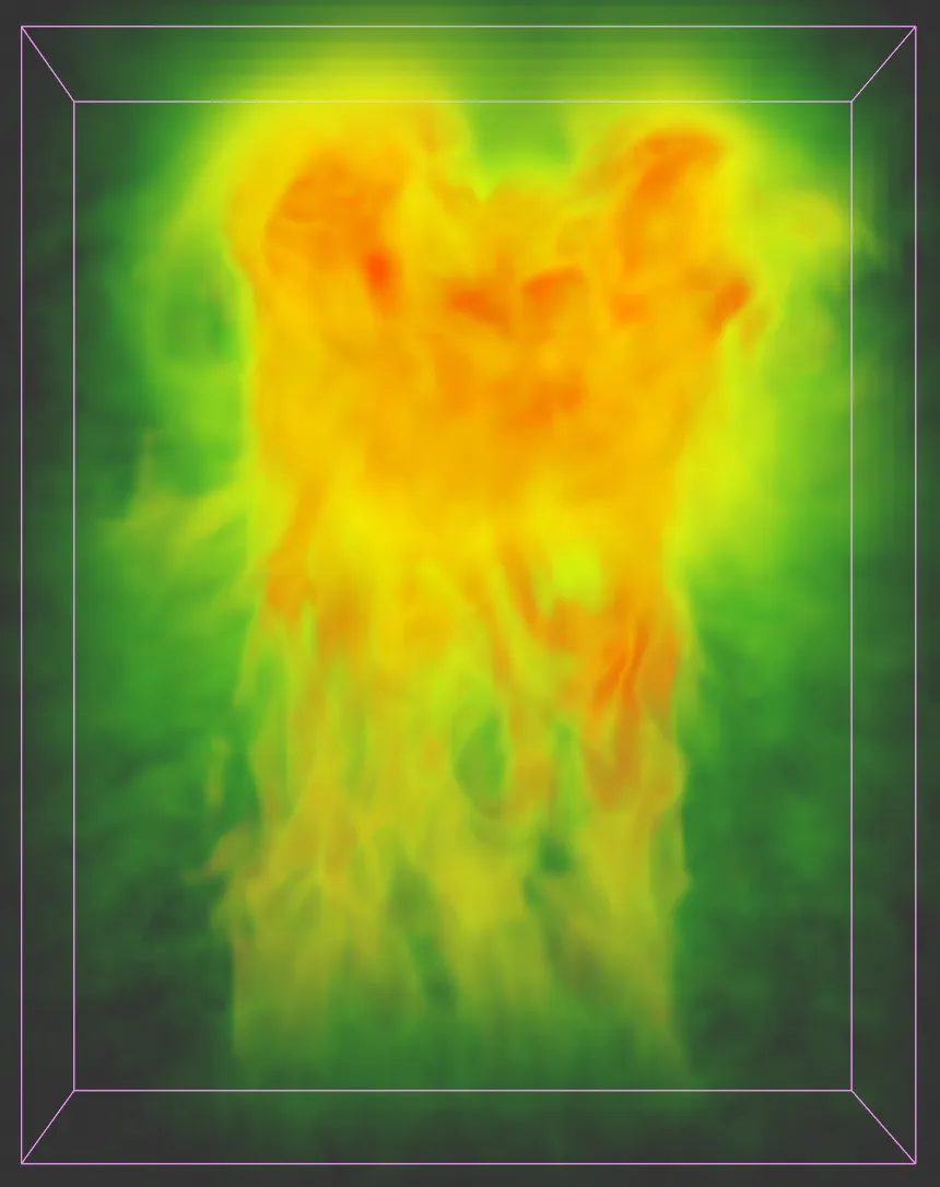
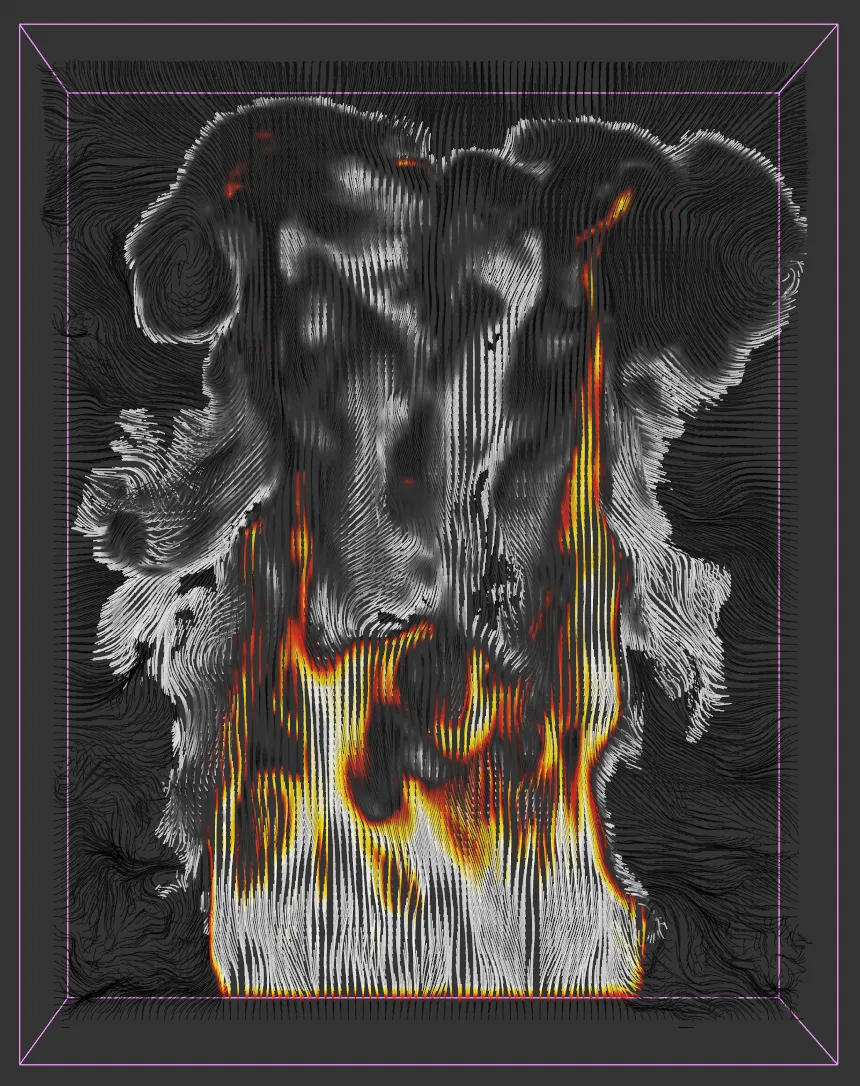
Temperature

The voxel temperatures are shown.

Display set to Temperature.

Smoke

Displays the smoke channel.

Display set to Smoke.

Fuel

Displays the fuel channel.

Display set to Fuel.

Fuel + Smoke

Both fuel and smoke are shown.

xpExplosiaFX_Display_Fuel and Smoke.png

Display set to Fuel + Smoke.

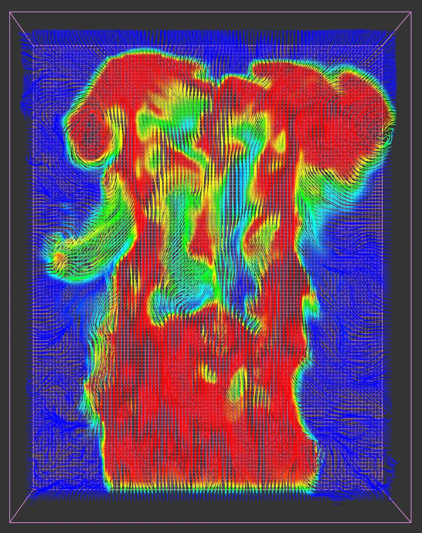
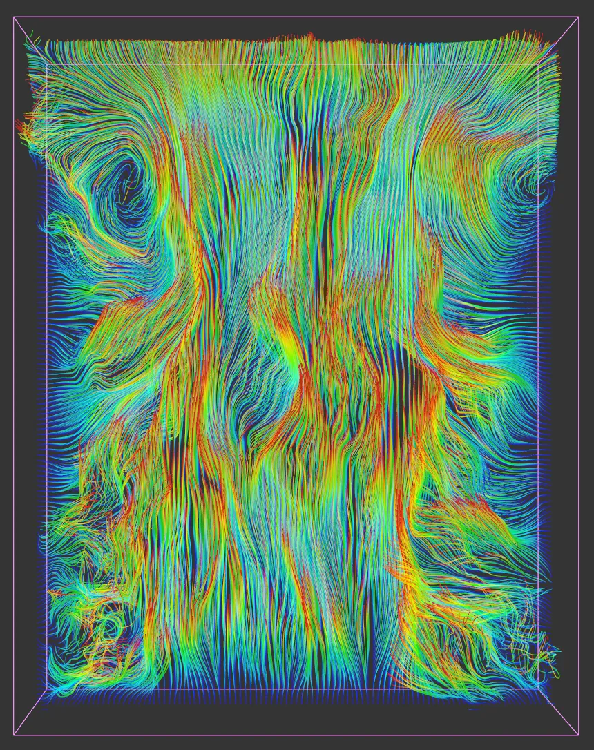
Velocity

In this mode, the actual flow vectors in the voxels are shown.

The same gradients are also used for the Speed channel.

Speed

The speed channel is shown.

It uses the same gradients as the Velocity channel.

Color

No gradients are available for this channel.

To use it, first check Color in the solver settings (Solver tab).

Then the color which is used is determined by the xpExplosiaFX Source tag.

Mode

Set as Slices, by default, the other options are: Off, Grid and Center Slice.

Off

The display is turned off and nothing will be seen if the simulation is run.

Slices

The display is composed of a number of slices and the detail can be adjusted by altering the Slices parameter.

The more slices, the more detailed the result, but it will be slower to run.

With Mode set to Slices and a Slices value of 18, with a Resolution of 64.

The Slices value is increased to 512 in this second image; the Resolution remains at 64.

Grid

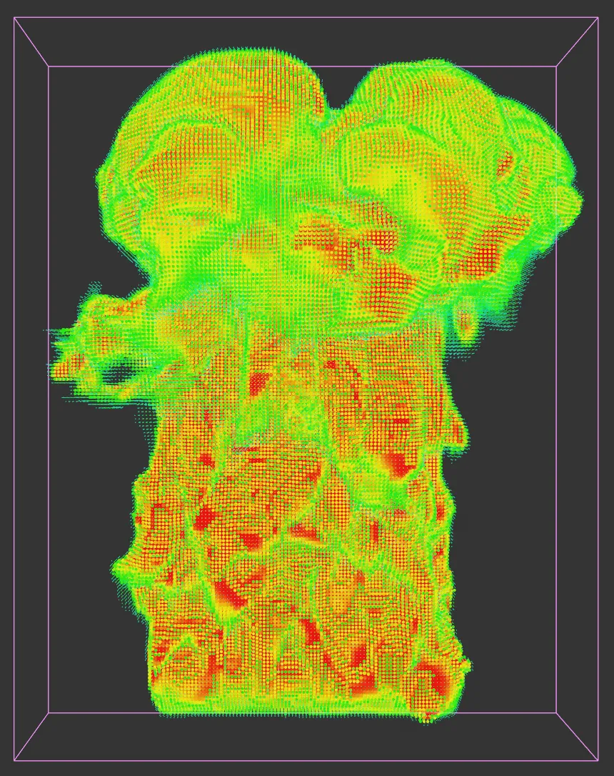
In this mode, each voxel is colored as required, giving rise to a grid of discrete dots rather than a continuous display.

This mode is faster than Slices but much less detailed.

You can control the level of detail with the Voxel LOD slider.

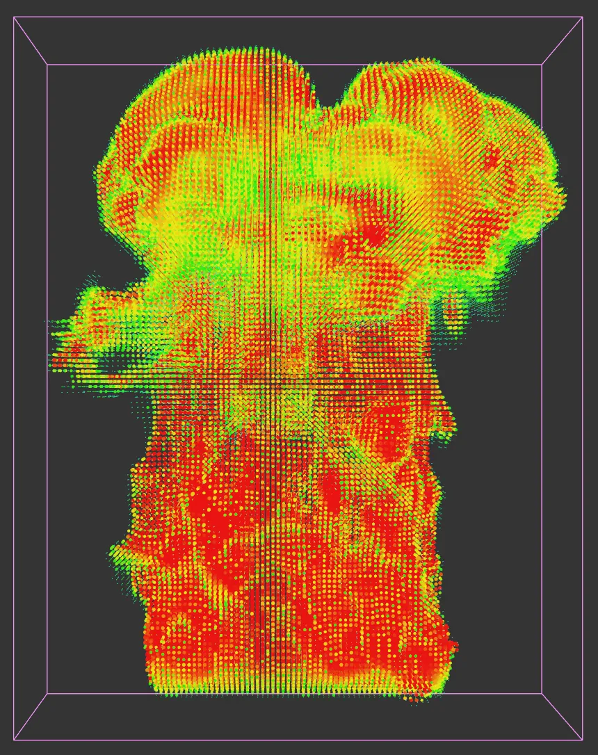
The Mode is now set to Grid, with a Voxel LOD value of 100%.

Voxel LOD raised to 150%.

Center Slice

One single slice is used from the center of the source object.

A very fast mode but without much detail.

Grid

Set as Bounds, by default, this menu controls how the solver object is displayed.

The alternative settings are: None, Voxels, Back and Base.

None

Only the adaptive bounds of the solver are displayed, unless those are also disabled.

Bounds

Only the bounding box of the solver and the adaptive bounds are shown.

Voxels

Each voxel is displayed as a small cube.

Back

A grid showing the voxel size is drawn on the furthest wall of the solver from the camera.

Base

A grid showing the voxel size is drawn on the base of the solver.

Bounds Color

The color used to draw the adaptive bounds.

Show Adaptive Bounds

Regardless of the selected option in Grid, if this setting is unchecked the adaptive bounds are not drawn.

Interpolate

If checked, colors between neighboring voxels are interpreted.

If unchecked, colors are shown as discrete voxels, giving a blocky appearance.

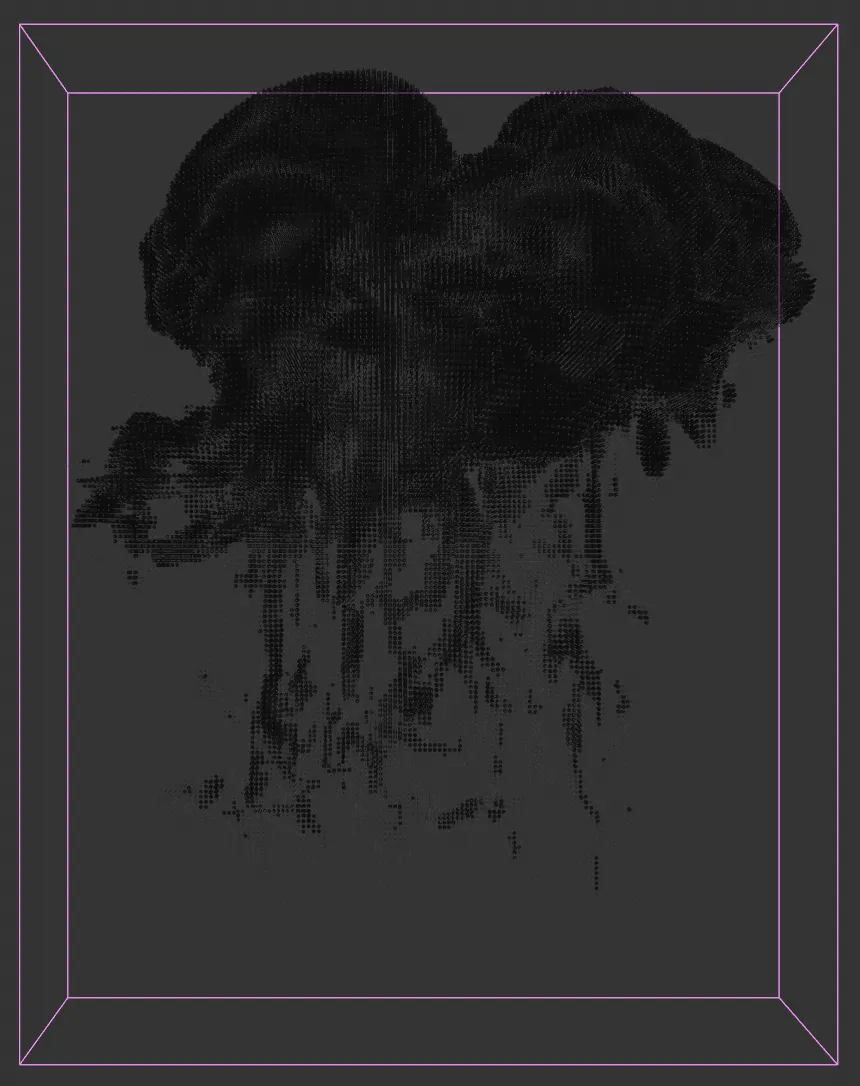
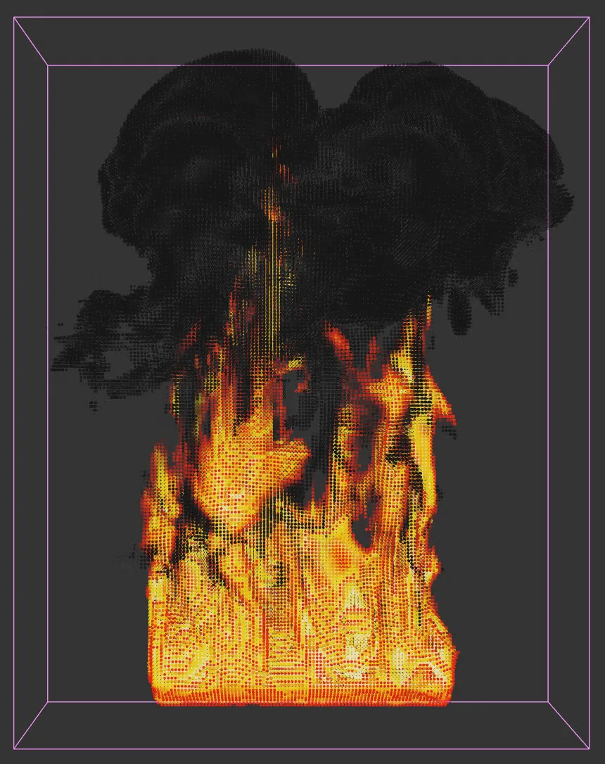
Trail Display

With these settings, a trail (not an X-Particles trail, as in the xpTrail object) is drawn to show changes in each voxel over time.

This gives you much more information about how temperature or other parameters are changing within the solver.

Display set to Temperature, with Trail Color disabled.

Display is now set to Fuel + Smoke, again with Trail Color disabled.

This final image shows Display set to Fuel + Smoke, but with Trail Color enabled.

Display Trails

Check this box to display the trails.

Show Trails Only

If this box is checked, only the trails are displayed, so the temperature, smoke, etc. displays are not shown.

Trail Color

If this box is checked, the trail color is taken form the Trail Color gradient, which appears.

If it is unchecked the trail color comes from the gradient used to color the display (that is, the Smoke Color gradient when Display is set to Smoke and so on).

Trail Color

This gradient is only visible when the Trail Color setting is enabled.

In that case, the trail colors are taken from this gradient.

Draw

This menu determines where the trails are drawn.

The options are the three orthographic planes XY, ZY and XZ, plus Voxels, where a trail is drawn for each voxel (within the adaptive bounds, if Adaptive Bounds is enabled, or within the entire solver if not).

Offset

By default, if Draw is set to one of the orthographic planes, the trails are drawn in the center of the adaptive bounds (or the center of the whole solver if Adaptive Bounds is disabled).

You can offset the drawing plane from the center by using this control.

This has no effect if Draw is set to Voxels.

Trail Length

The length of the trails in scene units.

Transparency

The overall transparency of the display can be altered using this setting.

Slices

The number of slices to take through the simulation if Mode is set to Slices.

Resolution

The resolution of the display.

The higher it is, the more detailed the display, but the slower it is to be drawn.

If you increase this too much, it will slow the simulation down significantly.

Only available if Mode is set to Slices or Center Slice.

Voxel LOD

The level of detail of the voxel display.

Only available if Display is set to Velocity or Mode is set to Grid.

Display Color sections

Each display type will have its own group of settings but in some cases these are identical in function between different displays.

Min Opacity, Max Opacity

These values control where along the opacity gradient the opacity value is taken from.

These settings are available for the temperature, fuel and smoke displays.

Color and Opacity Gradients

All display types except Color have two gradients, one for color and one for opacity.

There are separate pairs of gradients for each parameter option in Display, apart from Velocity and Speed, which share the same gradients, and Color, which doesn’t have any.

Temperature Color settings

In addition to the gradients, the temperature display has the following settings.

Color Mode

This menu determines whether the colors are controlled by blackbody radiation (Blackbody) or can be set manually (Manual).

If you choose Blackbody, the temperature color gradient is not available because the colors are derived from the standard blackbody color spectrum.

Additional settings then become available.

Blackbody Gradient

The color gradient used.

It cannot be edited directly, but will be altered if you change the Power, Min Temperature or Max Temperature settings.

Temp Transparency

Controls the overall transparency of the temperature display.

Power

The power of the blackbody radiation.

Reducing this value will shift the blackbody gradient to the left (you can see this gradient updating as you change this value).

Min Temperature, Max Temperature

These values will shift the blackbody gradient to the left or right and alter the temperature display accordingly.

Smoke display settings

There is only one additional setting here.

Smoke Transparency

This setting controls the overall transparency of the smoke.

Fuel display settings

These settings are identical to the temperature display settings above; please refer to that section for details.

The only difference is that, by default, the fuel display mode is set to Blackbody.

Velocity and Speed display settings

These displays share the same settings.

There are two additional settings.

Speed Min, Speed Max

These values determine where, on the Speed Color gradient, the color is sampled (and the seam for the Speed Opacity).

If the voxel speed is at or lower than Speed Min, the color is taken from the left-hand end of the gradient; if it is at or higher than Speed Max, it is taken from the right-hand end.

Fields tab

You can use the Fields options to control where xpExplosiaFX operates.