Mapping

The Mapping tab drives a modifier’s parameters from live particle data, so a setting changes per particle and over the course of the simulation instead of holding one fixed value.

Every full NeXus modifier carries a Mapping tab in Properties ▸ Physics, alongside Object Properties, Groups Affected and Falloff. The forces (nxGravity, nxWind, nxTurbulence and the rest) all have it, as do the simulation modifiers, the nxMesher generator and nxUpres. The lighter object-type modifiers do not: nxEmitter, nxCollider, nxGroup, nxGenerator, nxTrail, nxCache and nxFalloff have no Mapping tab.

Each entry in the tab is a layer. A layer routes one particle-data source into one modifier parameter: it reads the chosen particle property and uses it to modulate the chosen setting. The Mapping curve then shapes exactly how the source value maps onto the parameter value.

If a modifier has no mappable parameters the tab reads No mappable parameters and there is nothing to add.

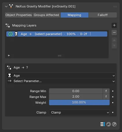
The Mapping tab on nxGravity, with one Age layer added

The Mapping tab on nxGravity. One layer has been added, keyed to the particle Age. The top half is the Mapping Layers list, and the box below holds the selected layer’s settings.

Mapping Layers

The top of the tab is the Mapping Layers list. Add, select, reorder and remove your layers here.

Add a layer

Click the + button to open the Add Mapping Layer menu, then pick the particle-data source the new layer is keyed by. The layer is created reading that source. You can change the source later from the layer’s settings.

There are twenty basic particle-data sources, available on every Mapping tab:

Age, Color (Brightness), Color R, Color G, Color B, Distance, Document Time, Fluid Density, Fuel, Granular, Group, ID, Life, Mass, Radius, Scale, Smoke, Speed, Temperature and Vertex Weight.

Some modifiers add their own sources to the bottom of this menu, grouped under their own headings, so the exact list depends on which modifier you are mapping.

The list

You can have as many layers as you wish. Each row shows a summary of the layer: its source, an arrow, the parameter it drives, then its weight, range and clamp mode. The check box at the start of each row is the layer’s Enabled toggle. Turn a layer off to suspend it without deleting it.

Select a layer to open its full settings in the box below.

Reorder and remove

The buttons beside the list remove the selected layer (-) and move it up or down. Order the layers to control how stacked mappings on the same parameter combine.

Layer settings

Selecting a layer opens its settings. The heading restates the routing as source → parameter so you can see at a glance what the layer does.

Source

The particle data this layer reads. It defaults to the source you picked when adding the layer. Open the menu to change it to any of the available particle-data types.

For example, set the source to Age to drive a parameter from how old each particle is, or to Speed to drive it from how fast the particle is moving.

Layer

On the layer-stack modifiers (nxTurbulence, nxScale, nxSpeed, nxSpin, nxDirection, nxLimit and nxColor) an extra Layer menu appears. These modifiers hold their own stack of layers, so this menu picks which of those layers the mapping targets. Modifiers without a stack do not show this control.

Parameter

The modifier parameter this layer modulates, chosen from the Parameter menu (shown with a forward arrow). The available parameters depend on which modifier you are mapping, and on some modifiers they are grouped under headings.

Until you pick one the menu reads Select Parameter… and the layer does nothing.

Range Min, Range Max

These set the span of source values the mapping reacts to. The Mapping curve is applied across this range: a source value at Range Min sits at the left of the curve, and a source value at Range Max sits at the right.

For a source such as Age, a Range Min of 40 and a Range Max of 50 means the curve affects each particle only while it is between 40 and 50 frames old.

For the time-based sources (Age, Life and Document Time) the range is entered in the NeXus time system, with a per-field frames or seconds toggle (the f or s button beside each field). It defaults to a Range Min of 0 and a Range Max of 2. For every other source the range is a plain value pair, defaulting to 0 to 1.

Weight

The blend strength of this layer, as a percentage. Defaults to 100%, applying the mapping in full. Lower it to blend the mapped value back toward the parameter’s own fixed value, so at 50% the parameter lands halfway between its base setting and the fully mapped result.

Clamp

Controls what happens when a particle’s source value falls outside the Range Min to Range Max span. Set as Clamp, by default. The alternatives are Cycle and Continue.

Clamp: hold the mapping at the start or end value once the source passes the edge of the range.
Cycle: wrap the source back through the range and repeat it in a continuous loop.
Continue: pass source values outside the range through unmodified, instead of clamping them to the edge.

Mapping

The curve that defines how the source value maps onto the parameter. It is the heart of the tab.

The horizontal X axis is the chosen source, with 0.0 at Range Min and 1.0 at Range Max. The vertical Y axis is a multiplier on the parameter, so at 1.0 the parameter takes its full value and at 0.0 it takes none of it.

With the default straight line the parameter rises evenly across the range. Edit the curve to shape that response: a downward line makes the parameter fall off across the range, and a curve that rises then falls makes it grow and then shrink.

Because the curve is a static graph, you can read off how a parameter behaves at any point in the range without playing the scene. Halfway along an Age range, a curve value of 0.5 means the particle gets half the parameter’s value at that age.

Once the source, parameter and range are set, editing this one curve is enough to build very different behaviors from the same layer.

Worked example: a surface-tension field

Mapping is easiest to understand from a real setup. This example drives an nxFluids liquid’s Surface Tension per particle from a spatial field, so the tension is zero at the center of an influence sphere and rises smoothly to full at its edge. Download the scene and open it in Blender 5.1 to follow along.

The scene playing in the viewport: a fluid body whose per-particle surface tension is set by the mapped field.

Download: surface_tension_field.blend

The Surface Tension slider cannot read an object directly, so the value is routed through particle Color:

An empty, ST_Field_Center, marks the middle of the field. Move it to relocate the field.
An nxColor modifier with a single Distance from Object layer, keyed to ST_Field_Center over a distance of 0 to 1.2m, writes a radial 0 to 1 value into each particle’s Color: black at the center, white at the edge.
nxFluids runs a FLIP solve with a base Surface Tension of 60%. On its Mapping tab, one layer reads Color (Brightness) and drives Surface Tension across a range of 0 to 1. The effective per-particle tension becomes 60% of the radial value, so it is 0 at the center and about 60% at the edge.

The modifier order matters. nxColor must run before nxFluids so the mapped tension reads the current frame’s color.

To adapt it, match the emitter radius and the nxColor distance to resize the influence, raise the nxFluids Surface Tension slider to change the maximum, and edit the Mapping curve or the color ramp to reshape the falloff.